Introduction of Statistical Data

Introduction of Statical Data:

Besides textual and tabular presentations of statistical data, the third and perhaps the most attractive and commonly used popular modem device to exhibit any data in a systematic manner is to represent them with suitable and appropriate diagrams and pictures.

The usual and effective means in this context are: graphs, charts, pictures, etc. and they are really and surely capable of depicting some important features of the data which they individually are not able to exhibit. Selection of the appropriate diagram actually depends on the nature of the raw data available and the purpose or the area in which it will be applied. However, only certain limited information can be supplied through a particular diagram and as such each diagram has certain specific limitations of its own.

A few commonly used diagrams applied on different occasions in various disciplines today are the line diagram, bar diagram, ogive, pie dia­gram and the pictogram (as prescribed in the syllabus).

It may be noted that diagrammatic represen­tations of statistical information is appealing to the eyes. Hidden facts may also be detected once such information are presented graphically. Further, graphs of statistical data clearly bring out the relative importance of different figures, the trend or tendency of the values of the variables involved can be studied too.

Line Diagrams:

This kind of a diagram becomes suitable for representing data supplied chronologically in an ascending or descending order. Usually, it shows the behaviour of a variable over time. Successive values of a variable at different periods or places are plotted as separate points on a two dimensional plane and the locus of all those points joined together form a continuous line segment, called line diagram.

While tracing out such a diagram, the usual convention is to show the successive values of the variable under study along the vertical axis in an increasing order and the time dimension along the horizontal axis. It should carefully be noted that none of the two axes be too long or too short with respect to each other.

This is very much necessary mainly to avoid unpredictable and wide fluctuations in the given values of the variable. The origin or the (0, 0) point at the left hand comer should clearly be mentioned so as to discard wrong impression on the process of drawing.

Two or more (but finite number of) line segments can also be drawn on the same quadrant when information on different variables over the same period or time are simultaneously represented using the same unit of measurement along the same axis. We can thus draw a number of line- diagrams for different data series on the same quadrant.

They can distinctly and attractively be displayed on a screen for presentation with various colourful lines. When the values of the variable under consideration change at a constant rate over the same successive time intervals, the diagram will take the shape of a straight line. Other-wise, it will represent various concave, convex or irregular curves when viewed from the origin.

Let us now represent a common line diagram below:

Example:

Line diagrams showing total values of Exports and Imports during 1987-96 have been presented in Fig. 7.1. This figure has been drawn on the basis of data shown in Table 7.4.

Two separate line diagrams showing fluctua­tions in the values of exports and imports of India during (1987—96) are shown below:

In the diagram drawn above the successive years from the table are shown horizontally and the corresponding values of export and import are shown vertically and the points are located separately on the plane from the middle of the respective years and the lacus of those points exhibit the trend along the line diagrams.

Bar Diagrams:

It is another well-known useful statistical weapon to represent raw data decently. This device is applied specially in a situation where the given data can be classified on the basis of a non- measurable criterion e.g., standards of college education in different states of India at the present time.

This is very often called cross-section data. More precisely, a bar graph is formed as a collection of rectangles having the same width or breadth placed successively at equal distance. Practically, the height of each bar placed vertically represents the value of the variable on the identical class interval shown horizontally.

Usually, these bars are placed either vertically on the horizontal axis or horizontally on the vertical axis and they are thus known as vertical bar chart or horizontal bar chart. Conventionally vertical bar charts are formed with the time series data.

Actually speaking, no formal rule as to how much space to be given in between the two bars is there. If necessary, no space in between two bars can be given. In some other cases, suitable and reasonable gaps in-between two bars may also be allowed.

Let us imprint simple and suitable examples of bar diagrams be­low:

(a) Simple Vertical Bar Diagram:

Volume of population in a number of states in India in 2001 is given below—represents the data with the aid of vertical bars.

Fig. 7.2 Shows population of a number of 5 States in India in a particular year (2001):

(b) Horizontal Bar Diagram:

Volume of production and profit of five different organisations operating under a particular industry with separate productive capacities are given below for the two successive years 2011 and 2012.

We represent the information through an ideal bar diagram. Here Fig. 7.3 is drawn below on the basis of Table 7.6. We have chosen this horizontal bar diagram to facilitate comparison of perfor­mances of 5 organisations for the years 2011 and 2012, respectively.

Horizontal bars show production (in thousands) and profit (Rs. thousand) of five organisations of India in the financial year 2011-12.

(c) Multiple or Component Bar Diagram

These diagrams are used in a situation where two or more related categories are to be compared simultaneously.

Consider the following example:

Labour employment and their percentages in 2000 and 2010 in a factory is given below. Repre­sent them in terms of multiple or component bar diagrams.

Component bar diagrams show number of labourers of different categories and their respec­tive percentages for the years 2000 and 2010.

Pie Diagram:

It is another effective statistical device to represent quantitative data obtainable on many occasions simply and diagrammatically. When the various parts of the values of a variable possesses different properties then to express the inherent relationship among them and also with the aggregate value of the variable, pie diagram possibly is the best device.

Here, the aggregate value of the variable is expressed as the total area of a circle with a reasonable radius. The entire area in the circle is subdivided into a number of parts by several radii which are separately related to the total area of the circle and also maintain the same proportional relation with the angle at the centre.

For drawing it correctly, we convert the particular given values of the variable as a percen­tage of the total value of the variable. As the angle at the centre is 360°, it is supposed to express 100 p.c. value of the variable where 1 p.c. value of the variable is equivalent to an angle of 3.6° at the centre.

We can thus easily convert the individual given values of the variable into the required angles at the centre. Then we draw a complete circle taking any standard radius and put the angles found from the numerical exercise separately at the centre. Each separate part in the circle signifies a particular section of the data. Let us represent a simple pie diagram below constructed with the usual method prescribed and followed for its computation by converting the following information into that diagram.

Example:

Expenditure incurred by the Planning Commission of India on Education in the last 5-year economic plan.

Table 7.8(A): Educational Expenditure in the Last Five-year Economic Plan:

Let us first convert the given data into respective percentages and then into the required angles to be shown at the centre in two more co­lumns and represent them in the following way:

Here, angle at the Centre = Percentage x 3.6.

Pie diagram drawn below on the basis of Table 7.8 (B) shows expenditure on education at various stages in the last 5-year economic plan.

Ogive or Cumulative Frequency Polygon:

An ogive is another statistical tool primarily used for finding out different quartiles in a distribution. From such a device we can also identify the number of observations lying above or below a certain value of the concerned variable.

This kind of a diagram is drawn for a fre­quency distribution of a continuous variable in terms of cumulative frequencies of both the types (more than or less than type). While drawing this diagram we consider the given values of the variable horizontally and the corresponding cumulative frequencies (of either type) vertically.

Cumulative frequency of less than type is zero for the lowest given value of the variable and similarly cumulative frequency of greater than type is zero for the highest value of the variable considered. Using the data available from a production organisation, Ogives of both the types are drawn below for our ready reference.

Ogives (of both the types) drawn on the basis of the above data and determination of the median wage:

Here, being the middle-most value of the given wage rates, the median wage is found OB (= Rs. 52) because only at this wage rate the two cumulative frequency curves intersect at point A representing two cumulative frequencies (less-than and greater-than) of both the types exactly equal (AB = 25) with each other. Hence, the median wage is OB = Rs. 52.00.

Measure of Disperson

What is Measures of Dispersion?

Measures of dispersion measure how spread out a set of data is.

Variance and Standard Deviation

The formulae for the variance and standard deviation are given below. m means the mean of the data.

Variance	=	s2	=	S (xr - m)2
				n

The standard deviation, s, is the square root of the variance.

What the formula means:
(1) xr - m  means take each value in turn and subtract the mean from each value.
(2) (xr - m)2  means square each of the results obtained from step (1). This is to get rid of any minus signs.
(3)  S(xr - m)2  means add up all of the results obtained from step (2).
(4) Divide step (3) by n, which is the number of numbers
(5) For the standard deviation, square root the answer to step (4).

Example

Find the variance and standard deviation of the following numbers: 1, 3, 5, 5, 6, 7, 9, 10 .

The mean = 46/ 8 = 5.75

(Step 1): (1 - 5.75), (3 - 5.75), (5 - 5.75), (5 - 5.75), (6 - 5.75), (7 - 5.75), (9 - 5.75), (10 - 5.75)
= -4.75, -2.75, -0.75, -0.75, 0.25, 1.25, 3.25, 4.25

(Step 2): 22.563, 7.563, 0.563, 0.563, 0.063, 1.563, 10.563, 18.063

(Step 3): 22.563 + 7.563 + 0.563 + 0.563 + 0.063 + 1.563 + 10.563 + 18.063
= 61.504

(Step 4): n = 8, therefore variance = 61.504/ 8 = 7.69 (3sf)

(Step 5): standard deviation = 2.77 (3sf)

Adding or Multiplying Data by a Constant

If a constant, k, is added to each number in a set of data, the mean will be increased by k and the standard deviation will be unaltered (since the spread of the data will be unchanged).

If the data is multiplied by the constant k, the mean and standard deviation will both be multiplied by k.

Grouped Data

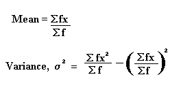
There are many ways of writing the formula for the standard deviation. The one above is for a basic list of numbers. The formula for the variance when the data is grouped is as follows. The standard deviation can be found by taking the square root of this value.

Example

The table shows marks (out of 10) obtained by 20 people in a test

Mark (x)	Frequency (f)
1	0
2	1
3	1
4	3
5	2
6	5
7	5
8	2
9	0
10	1

Work out the variance of this data.

In such questions, it is often easiest to set your working out in a table:

fx	fx2
0	0
2	4
3	9
12	48
10	50
30	180
35	245
16	128
0	0
10	100

Sf = 20
Sfx = 118
Sfx2 = 764

variance =  Sfx2  - ( Sfx )2
                      Sf      (  Sf  )2
 =  764  -  (118)2
     20       ( 20 )2
 =  38.2 - 34.81 = 3.39

Quartiles

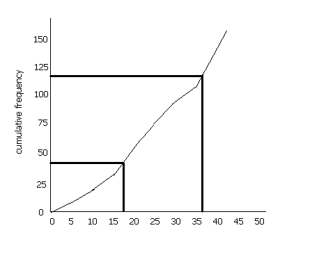
If we divide a cumulative frequency curve into quarters, the value at the lower quarter is referred to as the lower quartile, the value at the middle gives the median and the value at the upper quarter is the upper quartile.

A set of numbers may be as follows: 8, 14, 15, 16, 17, 18, 19, 50. The mean of these numbers is 19.625 . However, the extremes in this set (8 and 50) distort the range. The inter-quartile range is a method of measuring the spread of the numbers by finding the middle 50% of the values.

It is useful since it ignore the extreme values. It is a method of measuring the spread of the data.

The lower quartile is (n+1)/4 th value (n is the cumulative frequency, i.e. 157 in this case) and the upper quartile is the 3(n+1)/4 the value. The difference between these two is the inter-quartile range (IQR).

In the above example, the upper quartile is the 118.5th value and the lower quartile is the 39.5th value. If we draw a cumulative frequency curve, we see that the lower quartile, therefore, is about 17 and the upper quartile is about 37. Therefore the IQR is 20 (bear in mind that this is a rough sketch- if you plot the values on graph paper you will get a more accurate value).

Permutation & Combination

PERMUTATIONS & COMBINATION

Permutations 

Suppose we want to find the number of ways to arrange the three letters in the word CAT in different two-letter groups where CA is different from AC and there are no repeated letters.

Because order matters, we're finding the number of permutations of size 2 that can be taken from a set of size 3. This is often written 3_P_2. We can list them as:

CA   CT   AC   AT   TC   TA

Now let's suppose we have 10 letters and want to make groupings of 4 letters. It's harder to list all those permutations. To find the number of four-letter permutations that we can make from 10 letters without repeated letters (10_P_4), we'd like to have a formula because there are 5040 such permutations and we don't want to write them all out!

For four-letter permutations, there are 10 possibilities for the first letter, 9 for the second, 8 for the third, and 7 for the last letter. We can find the total number of different four-letter permutations by multiplying 10 x 9 x 8 x 7 = 5040. 

To arrive at 10 x 9 x 8 x 7, we need to divide 10 factorial (10 because there are ten objects) by (10-4) factorial (subtracting from the total number of objects from which we're choosing the number of objects in each permutation). You can see below that we can divide the numerator by 6 x 5 x 4 x 3 x 2 x 1:

           10!     10!    10 x 9 x 8 x 7 x 6 x 5 x 4 x 3 x 2 x 1
10_P_4 = ------- = ---- = --------------------------------------
        (10 - 4)!   6!                     6 x 5 x 4 x 3 x 2 x 1

                        = 10 x 9 x 8 x 7 = 5040          

From this we can see that the more general formula for finding the number of permutations of size k taken from n objects is:

           n! 
n_P_k = --------  
        (n - k)! 

For our CAT example, we have:

          3!     3 x 2 x 1
 3_P_2 = ---- = ----------- = 6
          1!         1

We can use any one of the three letters in CAT as the first member of a permutation. There are three choices for the first letter: C, A, or T. After we've chosen one of these, only two choices remain for the second letter. To find the number of permutations we multiply: 3 x 2 = 6.

Note: What's a factorial? A factorial is written using an exclamation point - for example, 10 factorial is written 10! - and means multiply 10 times 9 times 8 times 7... all the way down to 1.

---

Combinations

When we want to find the number of combinations of size 2 without repeated letters that can be made from the three letters in the word CAT, order doesn't matter; AT is the same as TA. We can write out the three combinations of size two that can be taken from this set of size three:

CA   CT   AT

We say '3 choose 2' and write 3_C_2. But now let's imagine that we have 10 letters from which we wish to choose 4. To calculate 10_C_4, which is 210, we don't want to have to write all the combinations out!
Since we already know that 10_P_4 = 5040, we can use this information to find 10_C_4. Let's think about how we got that answer of 5040. We found all the possible combinations of 4 that can be taken from 10 (10_C_4). Then we found all the ways that four letters in those groups of size 4 can be arranged: 4 x 3 x 2 x 1 = 4! = 24. Thus the total number of permutations of size 4 taken from a set of size 10 is equal to 4! times the total number of combinations of size 4 taken from a set of size 10: 10_P_4 = 4! x 10_C_4.
When we divide both sides of this equation by 4! we see that the total number ofcombinations of size 4 taken from a set of size 10 is equal to the number of permutations of size 4 taken from a set of size 10 divided by 4!. This makes it possible to write a formula for finding 10_C_4:

               10_P_4      10!         10!
     10_C_4 = -------- = ------- = ----------
                 4!      4! x 6!    4!(10-4)!


               10 x 9 x 8 x 7 x 6 x 5 x 4 x 3 x 2 x 1
            =  --------------------------------------
                4 x 3 x 2 x 1  (6 x 5 x 4 x 3 x 2 x 1)


              10 x 9 x 8 x 7    5040
            = -------------- = ------ = 210
               4 x 3 x 2 x 1     24 

More generally, the formula for finding the number of combinations of k objects you can choose from a set of n objects is:

            n!
n_C_k = ----------
        k!(n - k)!

For our CAT example, we do the following:

          3!      3 x 2 x 1     6 
3_C_2 = ------ = ----------- = --- = 3
        2!(1!)    2 x 1 (1)     2

Pascal's Triangle

We can also use Pascal's Triangle to find combinations:

   Row 0                   1
   Row 1                 1   1
   Row 2               1   2   1
   Row 3             1   3   3   1
   Row 4           1   4   6   4   1
   Row 5         1   5  10   10  5   1
   Row 6       1   6  15  20   15  6   1

Pascal's Triangle continues on forever - it can have an infinite number of rows. Each number is the sum of the two numbers just above it. For the 1 at the beginning of each row, we imagine that Pascal's triangle is surrounded by zeros: to get the first 1 in any row except row 0, add a zero from the upper left to the 1 above and to the right. To get the 3 in row 4, add the 1 left and above to the 2 right and above.

To find the number of combinations of two objects that can be taken from a set of three objects, all we need to do is look at the second entry in row 3 (remember that the 1 at the top of the triangle is always counted as row zero and that a 1 on the lefthand side of the triangle is always counted as entry zero for that row).

Looking at the triangle, we see that the second entry in row 3 is 3, which is the same answer we got when we wrote down all the two-letter combinations for the letters in the word CAT.

   Row 0                   1
   Row 1                 1   1
   Row 2               1   2   1
   Row 3             1   3   3   1

Suppose we want to find 10_C_4? To use Pascal's Triangle we would need to write out 10 rows of the triangle. This is a good time to use a formula.

More generally, to find n_C_k ("n choose k"), just choose entry k in row n of Pascal's Triangle.

One of the hardest parts about doing problems that use permutations and combinations is deciding which formula to use.

DONE BY: IMZ 

Measures of Central Tendency

Measures of Central Tendency

Introduction

A measure of central tendency is a single value that attempts to describe a set of data by identifying the central position within that set of data. As such, measures of central tendency are sometimes called measures of central location. They are also classed as summary statistics. The mean (often called the average) is most likely the measure of central tendency that you are most familiar with, but there are others, such as the median and the mode.

The mean, median and mode are all valid measures of central tendency, but under different conditions, some measures of central tendency become more appropriate to use than others. In the following sections, we will look at the mean, mode and median, and learn how to calculate them and under what conditions they are most appropriate to be used.

Mean (Arithmetic)

The mean (or average) is the most popular and well known measure of central tendency. It can be used with both discrete and continuous data, although its use is most often with continuous data (see our Types of Variable guide for data types). The mean is equal to the sum of all the values in the data set divided by the number of values in the data set. So, if we have n values in a data set and they have values x₁, x₂, ..., x_n, the sample mean, usually denoted by  (pronounced x bar), is:

This formula is usually written in a slightly different manner using the Greek capitol letter, , pronounced "sigma", which means "sum of...":

You may have noticed that the above formula refers to the sample mean. So, why have we called it a sample mean? This is because, in statistics, samples and populations have very different meanings and these differences are very important, even if, in the case of the mean, they are calculated in the same way. To acknowledge that we are calculating the population mean and not the sample mean, we use the Greek lower case letter "mu", denoted as µ:

The mean is essentially a model of your data set. It is the value that is most common. You will notice, however, that the mean is not often one of the actual values that you have observed in your data set. However, one of its important properties is that it minimises error in the prediction of any one value in your data set. That is, it is the value that produces the lowest amount of error from all other values in the data set.

An important property of the mean is that it includes every value in your data set as part of the calculation. In addition, the mean is the only measure of central tendency where the sum of the deviations of each value from the mean is always zero.

When not to use the mean

The mean has one main disadvantage: it is particularly susceptible to the influence of outliers. These are values that are unusual compared to the rest of the data set by being especially small or large in numerical value. For example, consider the wages of staff at a factory below:

Staff	1	2	3	4	5	6	7	8	9	10
Salary	15k	18k	16k	14k	15k	15k	12k	17k	90k	95k

The mean salary for these ten staff is $30.7k. However, inspecting the raw data suggests that this mean value might not be the best way to accurately reflect the typical salary of a worker, as most workers have salaries in the $12k to 18k range. The mean is being skewed by the two large salaries. Therefore, in this situation, we would like to have a better measure of central tendency. As we will find out later, taking the median would be a better measure of central tendency in this situation.

Another time when we usually prefer the median over the mean (or mode) is when our data is skewed (i.e., the frequency distribution for our data is skewed). If we consider the normal distribution - as this is the most frequently assessed in statistics - when the data is perfectly normal, the mean, median and mode are identical. Moreover, they all represent the most typical value in the data set. However, as the data becomes skewed the mean loses its ability to provide the best central location for the data because the skewed data is dragging it away from the typical value. However, the median best retains this position and is not as strongly influenced by the skewed values. This is explained in more detail in the skewed distribution section later in this guide.

Median

The median is the middle score for a set of data that has been arranged in order of magnitude. The median is less affected by outliers and skewed data. In order to calculate the median, suppose we have the data below:

65

55

89

56

35

14

56

55

87

45

92

We first need to rearrange that data into order of magnitude (smallest first):

14

35

45

55

55

56

56

65

87

89

92

Our median mark is the middle mark - in this case, 56 (highlighted in bold). It is the middle mark because there are 5 scores before it and 5 scores after it. This works fine when you have an odd number of scores, but what happens when you have an even number of scores? What if you had only 10 scores? Well, you simply have to take the middle two scores and average the result. So, if we look at the example below:

65

55

89

56

35

14

56

55

87

45

We again rearrange that data into order of magnitude (smallest first):

14

35

45

55

55

56

56

65

87

89

Only now we have to take the 5th and 6th score in our data set and average them to get a median of 55.5.

Mode

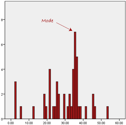
The mode is the most frequent score in our data set. On a histogram it represents the highest bar in a bar chart or histogram. You can, therefore, sometimes consider the mode as being the most popular option. An example of a mode is presented below:

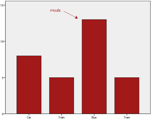
Normally, the mode is used for categorical data where we wish to know which is the most common category, as illustrated below:

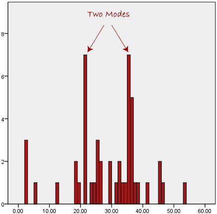
We can see above that the most common form of transport, in this particular data set, is the bus. However, one of the problems with the mode is that it is not unique, so it leaves us with problems when we have two or more values that share the highest frequency, such as below:

We are now stuck as to which mode best describes the central tendency of the data. This is particularly problematic when we have continuous data because we are more likely not to have any one value that is more frequent than the other. For example, consider measuring 30 peoples' weight (to the nearest 0.1 kg). How likely is it that we will find two or more people with exactly the same weight (e.g., 67.4 kg)? The answer, is probably very unlikely - many people might be close, but with such a small sample (30 people) and a large range of possible weights, you are unlikely to find two people with exactly the same weight; that is, to the nearest 0.1 kg. This is why the mode is very rarely used with continuous data.

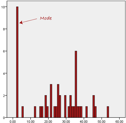
Another problem with the mode is that it will not provide us with a very good measure of central tendency when the most common mark is far away from the rest of the data in the data set, as depicted in the diagram below:

In the above diagram the mode has a value of 2. We can clearly see, however, that the mode is not representative of the data, which is mostly concentrated around the 20 to 30 value range. To use the mode to describe the central tendency of this data set would be misleading.

Skewed Distributions and the Mean and Median

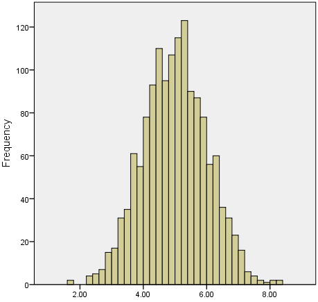
We often test whether our data is normally distributed because this is a common assumption underlying many statistical tests. An example of a normally distributed set of data is presented below:

When you have a normally distributed sample you can legitimately use both the mean or the median as your measure of central tendency. In fact, in any symmetrical distribution the mean, median and mode are equal. However, in this situation, the mean is widely preferred as the best measure of central tendency because it is the measure that includes all the values in the data set for its calculation, and any change in any of the scores will affect the value of the mean. This is not the case with the median or mode.

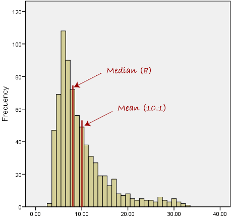
However, when our data is skewed, for example, as with the right-skewed data set below:

we find that the mean is being dragged in the direct of the skew. In these situations, the median is generally considered to be the best representative of the central location of the data. The more skewed the distribution, the greater the difference between the median and mean, and the greater emphasis should be placed on using the median as opposed to the mean. A classic example of the above right-skewed distribution is income (salary), where higher-earners provide a false representation of the typical income if expressed as a mean and not a median.

If dealing with a normal distribution, and tests of normality show that the data is non-normal, it is customary to use the median instead of the mean. However, this is more a rule of thumb than a strict guideline. Sometimes, researchers wish to report the mean of a skewed distribution if the median and mean are not appreciably different (a subjective assessment), and if it allows easier comparisons to previous research to be made.

Summary of when to use the mean, median and mode

Please use the following summary table to know what the best measure of central tendency is with respect to the different types of variable.

Type of Variable	Best measure of central tendency
Nominal	Mode
Ordinal	Median
Interval/Ratio (not skewed)	Mean
Interval/Ratio (skewed)	Median

Probability

Probability

What is Probability?

Probability is simply how likely something is to happen.

Whenever we’re unsure about the outcome of an event, we can talk about the probabilities of certain outcomes—how likely they are. The analysis of events governed by probability is called statistics.  

The best example for understanding probability is flipping a coin:

There are two possible outcomes—heads or tails.

What’s the probability of the coin landing on Heads? We can find out using the equation $P(H) = ?$.You might intuitively know that the likelihood is half/half, or 50%.  But how do we work that out?  Probability = 

In this case:

Probability of an event = (# of ways it can happen) / (total number of outcomes)

P(A) = (# of ways A can happen) / (Total number of outcomes)

Example 1

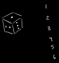
There are six different outcomes.

What’s the probability of rolling a one?

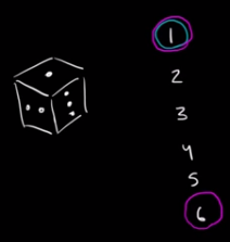
What’s the probability of rolling a one or a six?

Using the formula from above:

What’s the probability of rolling an even number (i.e., rolling a two, four or a six)?

Tips

• The probability of an event can only be between 0 and 1 and can also be written as a percentage.
• The probability of event $A$ is often written as $P(A)$.
• If $P(A) > P(B)$, then event $A$ has a higher chance of occurring than event $B$.
• If $P(A) = P(B)$, then events $A$ and $B$ are equally likely to occur.